Virus-X 3DM tutorial 2018
- Joanna Lange (Unlicensed)
- Tom van den Bergh
Intro
Welcome to the 3DM tutorial. A 3DM system is a data integration platform, we collect and integrate data about a protein superfamily.
Go to https://3dmjs.bio-prodict.nl and log in. From here you can navigate to different superfamily/family systems.
You have access to more than 24k systems, each containing from 2k to 300k sequences.
Protein detail page
For now we're going to work on a UniProt protein E2R0G7 (soon the same functionalities will be available for connected Virus-X proteins)
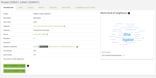
This page displays the most basic information about your protein, like gene name, description, species, etc.
The core identity is the sequence identity of the query protein to the subfamily template. Usually, the higher identity the higher the quality of the protein's alignment.
On the right you see a word cloud - which is a set the most abundant keywords annotated on the proteins most closely related to our protein of interest. It can give you an idea on what are the functions, classification, etc. of your protein.
Now click on the sequence tab - you'll see there how the sequence is aligned. The lowercase residues represent the residues that are not aligned (so called 'variable regions').
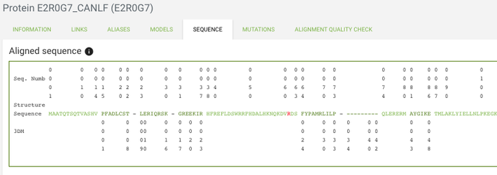
There are two different numberings displayed - the top one is the residue numbering which represents residue numbers in the sequence, while the bottom one are 3DM numbers, which represent the positions in the alignment - we use these number to unify the residue numbers across the whole superfamily, allow for per-residue data integration and simplify comparison of certain positions between different proteins.
If a residue is red that means that there is some additional data from the literature about it - can be mutations but also just mentions in the literature.
You can investigate in more detail these mentions/mutations in the mutations tab.

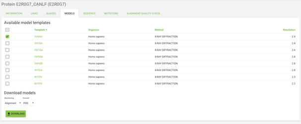
In the MODELS tab you can create a homology model for your sequence.
Back in the INFORMATION tab at the very bottom of the page there is a view in phylogenetic tree button, click on it and in the window that pops up click 'open'.
Your protein of interest is here marked with a red circle. The nodes in the tree are all the structural alignment templates and 50 extra proteins that were added to give you better idea of the protein in the context of the whole alignment.
Later, when the Virus-X proteins are added to the system you'll also be able to view a phylogenetic tree of all of these proteins.
Let's now again go back to the INFORMATION tab and click on the link in the aligned in subfamily field, show protein in subfamily alignment - the ID is the PDB id of the structure that was used as a template for the subfamily alignment.
Alignment page
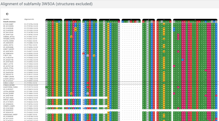
Now we're at the alignment where your protein of interest is aligned. The displayed residues are only residues that are aligned in the core regions - core regions is part of the alignment that is aligned across the whole superfamily.
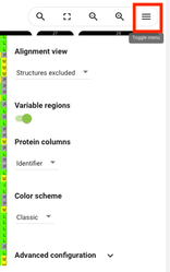
We can display the variable regions by clicking on the menu button on the top right from the alignment and clicking on the variable regions toggle.
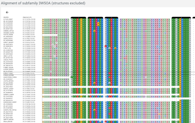
The lighter coloured residues are the variable regions and the bright-coloured ones are core regions. Keep in mind that only the aligned parts of the variable regions are displayed so you often don't see the full sequence in this view.
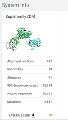
System info
Let's now have a look at the system info page - you can find a link in the menu on the left. This shows you an overview of the system, and gives you an idea of how much data there is.
Alignment statistics
Let's now navigate to the alignment statistics page, which you can access from the menu on the left side of the page.
Plots represent different kinds of data, e.g. ligand contacts, amino acid conservation, etc. mapped onto the alignment positions.
Next to each plot's title there is an i sign - if you mouse over it you can get a more detailed information about the data in the plot.
All plots have sliders which allow you to play around with value cut-offs of the displayed data.
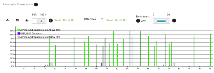
There is also a compare with dropdown menu - this allows you to display two kinds of data and investigate if there are any correlations.
Go to the amino acid conservation plot and choose DNA/RNA contacts from the compare with dropdown menu. To make the plot more readable, change the conservation cut-off to only display positions with conservation above 50% (the slider on the left).
If you scroll a bit to the right (around position 200) you'll see that positions with the most DNA/RNA contacts are also very highly conserved - that's exactly what we would expect.
Another thing you can do here is visualise this data in yasara - to do that click on the little button with a protein helix symbol  . You will be redirected to the visualize page, but don't do it for now, we'll get to it later.
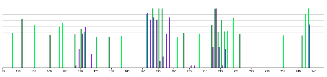
Alignment position page
You can also view data that's mapped onto a certain position in the alignment - the alignment position pages can be accessed in multiple ways, e.g.
- from the histograms on the alignment statistics page
- from the sequence tab on the protein detail page - click on a residue in the sequence, you'll be redirected to a residue page and from there you can go the alignment position page
- from the correlated mutations page - click a node in the network and on the right below 'Amino acid distribution' there's a link to the corresponding alignment position page
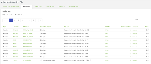
On the histogram scroll to the right and click on the bar for position 214. Now we can take a look around the alignment position page. Here in the different tabs you can see what data is mapped onto this position across all proteins in the 3DM systems. For example, in the mutations tab you can see all the mutations that we've found in the literature for this alignment position across all proteins in the system.
Visualize
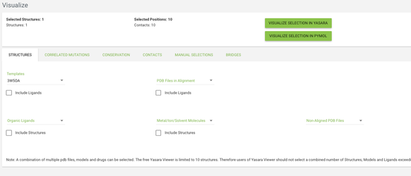
Go to the Visualize page from the menu, and click on the structures tab. From the templates menu select the 3W5OA structure - this is the template of the subfamily where our protein of interest is aligned. From the other tabs you can choose what data do you want to see mapped onto the structure - by default the residues with highest conservation and with highest correlated mutation score will be highlighted.
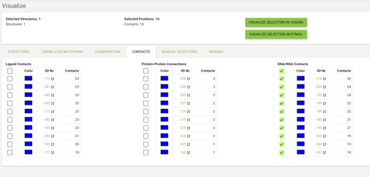
Go to the contacts tab and click on the checkbox in the top row in the DNA/RNA Contacts table (by clicking on the checkbox in the top row you toggle between selecting and deselecting all positions). Now click on the VISUALIZE IN YASARA button and a yasara scene with the selected data mapped onto the 3W5OA structure will be downloaded.
YASARA
Open the downloaded scene in YASARA. You can see that some parts of the backbone are green(ish) and some are gray - the gray color indicates that these residues fall in the variable regions, while green are core residues.
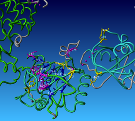
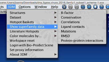
You can also access 3DM data from within yasara using our 3DM plugin - in the menu bar there is a '3DM' tab - there are numerous options of mapping your data onto the structure(s). Let's for example have a look at the mutation data. Go to 3DM > Show superfamily data > Mutations - now residues corresponding to alignment positions with the highest number of mutations are shown - you can see that they are mostly located in the pocket where you previously saw a lot of residues with DNA contacts. It makes sense that these residues are the ones that are most often mutated by researchers to investigate their function and the effect of mutations on DNA binding.

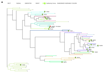
Phylogeny
Now click on the phylogeny item from the menu on the left. This shows an overall phylogeny tree where each node is one subfamily template. When you mouse over a subfamily ID you can display more information about the template structure.
Search options
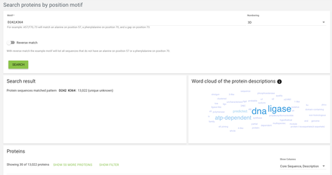
There are multiple ways to search proteins in a 3DM system. While most of them are quite straightforward and probably don't need to be explained, we'll have a closer look at the 'Search proteins by position motif' and 'Search proteins by sequence motif'.
These two search modes provide a similar functionality, the difference being that in the search by sequence motif the specified motif can appear on any position in the sequence.
In the case of search proteins by position motif, we're looking for specific motifs on specific positions - for example we might want to find all proteins that have an aspartate on alignment position 242 and a lysine on alignment position 364
Virus-X proteins
Virus-X proteins are proteins that are added to the system through the Virus-X pipeline, they're only accessible for the Virus-X users.
Follow this link to go to the list of Virus-X proteins in the DNA ligase system: DNA ligase
For now there is just one protein, but later on we'll be adding more proteins from the Bielefeld's webserver.
Advanced
Numbering schemes
You can simplify your work with the protein of interest even more by creating a custom numbering scheme - that will cause the alignment positions to be renumbered to match the residue numbering of your protein.
To do it you need to go back to the protein detail page of our protein of interest and click on the create numbering scheme button. You don't need to actually do it now, as we've already created a numbering scheme for this protein.
To switch between the different numbering schemes click on the dropdown menu in the numbering scheme at the top of the page. And don't worry, creating new numbering schemes doesn't erase the previously existing ones, so after creating a custom numbering scheme you can still switch to the original 3DM numbering or other numbering schemes that you created.
Subsets
If we want to analyse only some of the proteins present in the system - for example only the closest homologs of the query protein than we'll need the subsets functionality. We're going to create a subset of 100 closest proteins to our E2R0G7 protein. To do that we need to again go to the protein detail page E2R0G7 and click in the sequence tab.
Now click on the BLAST button which will redirect us to the BLAST page, change maximum number of hits to 100 and click search.
When the blast job is finished click on the yellow SUBSETS button on the right of the page header. Then click on NEW next to the subset name.
To create a subset you will need to select all proteins, and then click on the round + button - the selected proteins have now been added to the subset. To finish the subset creation you need to give a name of the new subset and click on SAVE & GENERATE - let's not actually do it, we've already generated one for this set of proteins.
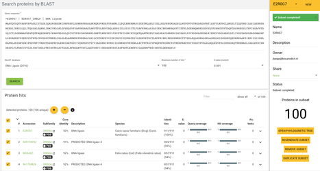
Now if we want to work only with these proteins we can select this subset in the subset field right below the system's name at the top of the page. Now all the data throughout the system will be only based on these 100 proteins - so for example correlated mutations, alignment statistics, etc.
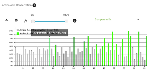
What we can also do is compare our small subset of proteins to the full dataset - to do this let's navigate again to the alignment statistics page and click on the custom plots tab.
Choose the two subsets 'Full dataset' and 'E2R0G7' and select 'Amin Acid Conservation' in the 'Data Types' field. Now click on generate.
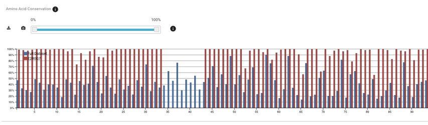
You can see on the plot that there are residues that are 100% conserved in the smaller subset of proteins while they don't have a significant conservation value in the full dataset.
Note that you can also create subsets from results from all the other searches not only BLAST search - these will be described in the next section.
Hotspots
You can also use 3DM to find hotspots - important residues, affecting e.g. protein specificity or thermostability.
What if you don't have a protein of interest?
Panel design - protein selection tool
This is a tool to facilitate the design of enzyme selection panels (for example based on the sequence diversity on the selected hotspots). For this you're gonna need a more advanced course.
If you want to know more about the advanced tools, you can ask us for more information or sign up for the course.
Please, send us feedback if you have any suggestions or if you think that something needs more clarification.
You can mail us or use the "Send feedback" form (linked on the bottom of the page)
Appendix
Correlation network and enrichment
Let's now go back to the website. Click on the correlated mutations item in the menu on the left. Now you see a network of correlated mutations - you can play around with the score cut-offs using the slider on the right. What you can also do is check if the positions involved in this network have any mutations with certain keywords assigned to them.
In the Literature & Mutations section on the right type 'activity' in the keyword field. A lot of residues in the network are now coloured with cyan - that means that there mutations described in literature associated with protein activity.
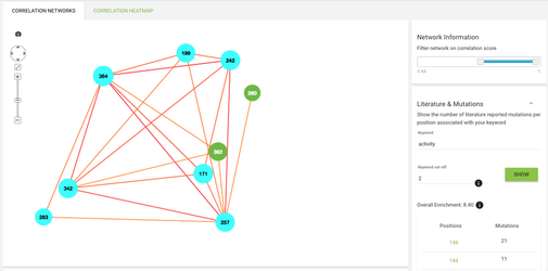
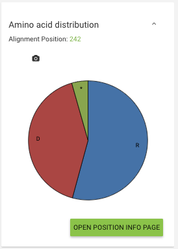
If you click on a node in the network you'll see on the right what residues are most abundant on this alignment position, and if you click on an edge between 2 positions you'll see a pie chart showing the correlating pairs of residues on the given positions.

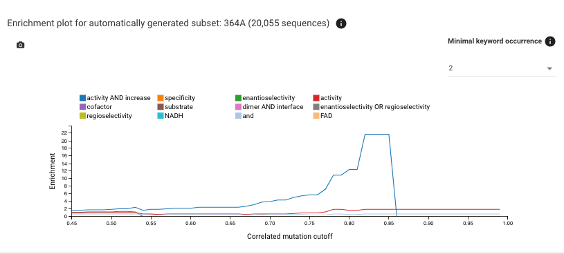
If you scroll down, you'll see enrichment plots - from these you get an overview of which mutation keywords are abundant on the positions in the correlated mutations network.
The plot below shows the same data but only for sequence that have an alanine on position 364 - for this plot always the position with the highest conservation is chosen.
'NADH' is the keyword with the most significant enrichment, that might mean that the residue might somehow influence NADH binding.